Data services for your favourite tools. Run reports or SQL queries.
It's now easy to automate access to multiple live data sets from our cloud data servers using your favourite tools like Excel, R, Matlab, Python, Grafana, and Google Sheets. Its easy to do and a lot easier than manually copying and pasting data, especially for repetitive analyses. Our data servers have full historic data since the start of the NEM in 1998 plus STTM and VICGAS, BOM etc. Using the data services feature you can easily access, all this without installing any software or any database drivers. Users can run the data services from anywhere: home, office or mobile.
NEOpoint
NEOpoint data service can be run from any machine connected to either the IES NEOpoint server or
customer's own NEOpoint server - useful if you want to report on private data. Link URL for NEOpoint data service uses Favourite path and can be found by
clicking on the "Get Links"  button.
NEOexpress
NEOexpress data service connects to the IES NEOexpress server and is accessible on any computer with an internet connection. It uses Report paths whereas NEOpoint uses a Favourite path. You can simply right click on any chart and select "Copy Service URL" to get the data service link.
QueryTool
Data service in QueryTool allows you to run SQL queries directly (compared to NEOpoint and NEOexpress which run reports). For examples of how to run the data service using QueryTool, please see section running SQL queries for each different tools below.
Excel
As with all the other tools data services allows you to load multiple data sets automatically. We have an XLSM file that demonstrates a simple case of loading 5 min price and demand from two separate reports. The macro is easy to modify to load any report, time period or instances. Excel sample
Excel expects web query data to be in XML format. You can either load it manually, or if this is something you do on a regular basis you may want to create a macro. The advantages of macros is that you can instantly load any number of live data sets and perform calculations on them all with the press of a button.
Running Reports
To start, open NEOpoint and run the required report and then click the “Links” button, select and copy the link. Sample XML link: https://www.neopoint.com.au/Service/Xml?f=104+Bids%5cRegion+Merit+Order+Stack+5min&period=Daily& from=2015-10-13&instances=Generator;NSW1§ion=0&key=***** An XML link has several parameters that you can customize.
- F – favourites object + selected report name
- Period – report period code
- From – report from date
- Instances – report instances
- Section – depends on the report but in most cases can be left as 0
- Key – NEOpoint login account API key
To manually load a result follow these steps:
- open a blank Excel worksheet
- click on the Data tab and click on “From Web”, in the dialog Address paste the URL you copied from NEOpoint, click GO then Import, set the location where you want the data to go
- that’s it – the data should appear in the spreadsheet
The big advantage of data services is automatically loading results. This makes it easy to create spreadsheets that with the click of a button will load several data sets and perform calculations. The macro text below shows how to load data automatically. You can simply copy the text for the macro and paste into your own copy of an Excel spreadsheet, modifying the URL as required. You can also set where you want the data to be loaded and load additional data sets in the same macro by repeating the XmlImport line with the required URL for each additional data set. To understand the macro we also need to explain two other lines of code:
- Every time you import XML data, Excel creates an “XMLMap” so in your macro you need to add some code to delete ALL the XMLMaps otherwise they will keep accumulating. That’s what the XmlMap.Delete line does.
- When data is imported it is marked as read only and hence you can’t load new data on top of it hence we add a “ClearContents” command to clear the contents of the cells you are about to import data into. You will need to adjust the range “G:H” to match the columns where you will be importing data.
The sample macro code is shown below.
Sub GetData1()

'
' Get prices and demand
'
For Each XmlMap In ActiveWorkbook.XmlMaps
                  XmlMap.Delete
        Next

Columns("G:H").ClearContents
ActiveWorkbook.XmlImport URL:= _
        "https://www.neopoint.com.au/Service/Xml?f=101+Prices%5CRegion+Price+5min&from=2021-10-28+00%3A00&period=Daily&instances=NSW1§ion=-1&key=XXXXXXX" _
        , ImportMap:=Nothing, Overwrite:=True, Destination:=Range("$G$1")

Columns("J:N").ClearContents
ActiveWorkbook.XmlImport URL:= _
        "http://www.neopoint.com.au/Service/Xml?f=products.iesys.com%5cDemand+5min&period=Daily&from=2016-10-21&instances=NSW1§ion=-1&key=XXXXXXX" _
        , ImportMap:=Nothing, Overwrite:=True, Destination:=Range("$J$1")


End Sub
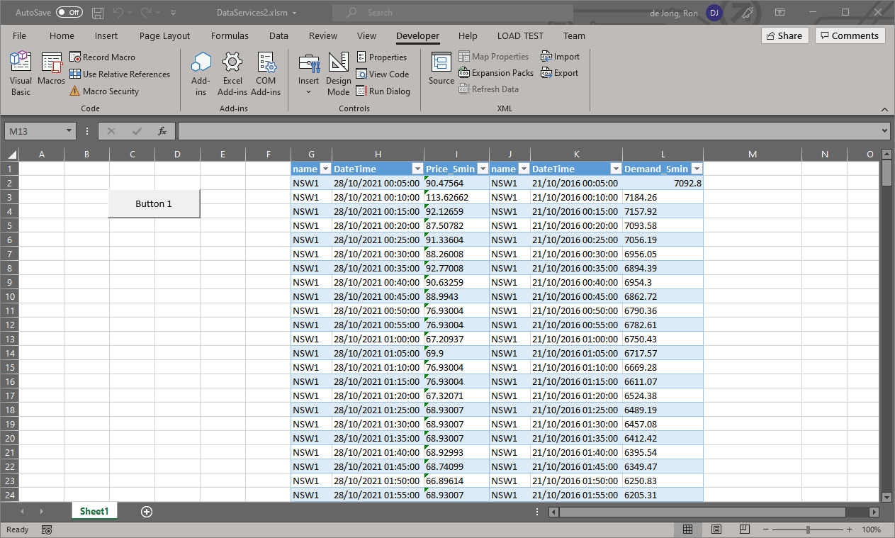
If the above macro is linked to a button and the button is clicked it will load the report results into the spreadsheet as shown below.
Running SQL queries
The sample code below shows how to write a macro that loads data from an SQL query.
Sub LoadData()

'Clear the workbook, adjust based on the columns your query uses
Columns("A:Z").ClearContents

'Put your Query here, ensure that multi line queries are joined together as separate strings (as in the following example)
Query = "select `SETTLEMENTDATE`, `RUNNO`, `REGIONID`, `PERIODID`, `RRP`, `EEP`," & _
"`INVALIDFLAG`, `LASTCHANGED`, `ROP`, `RAISE6SECRRP`, `RAISE6SECROP`, " & _
"`RAISE60SECRRP`, `RAISE60SECROP`, `RAISE5MINRRP`, `RAISE5MINROP`, " & _
"`RAISEREGRRP`, `RAISEREGROP`, `LOWER6SECRRP`, `LOWER6SECROP`, `LOWER60SECRRP`, " & _
"`LOWER60SECROP`, `LOWER5MINRRP`, `LOWER5MINROP`, `LOWERREGRRP`, `LOWERREGROP`, " & _
"`PRICE_STATUS` from mms.tradingprice where SETTLEMENTDATE between '2018-11-01' and '2018-11-02' limit 0, 10000"

'Put your API key here
apikey = "XXXXXXXXXXXXXXXX"

'Make POST Request
Set objHTTP = CreateObject("MSXML2.ServerXMLHTTP")
Url = "https://www.neopoint.com.au/data/query"
objHTTP.Open "POST", Url, False
objHTTP.setRequestHeader "Content-Type", "application/x-www-form-urlencoded"
objHTTP.Send ("query=" & Query & "&key=" & apikey & "&format=csv")

'get response text
resp = objHTTP.responseText

'Write to File
If objHTTP.Status = "200" Then
    Lines = Split(resp, Chr(10))
    For r = LBound(Lines) To UBound(Lines)
        Values = Split(Lines(r), ", ")
        For c = LBound(Values) To UBound(Values)
            Cells(r + 1, c + 1).Value = Values(c)
        Next c
    Next r
Else
    MsgBox "The POST request failed"
End If

End Sub
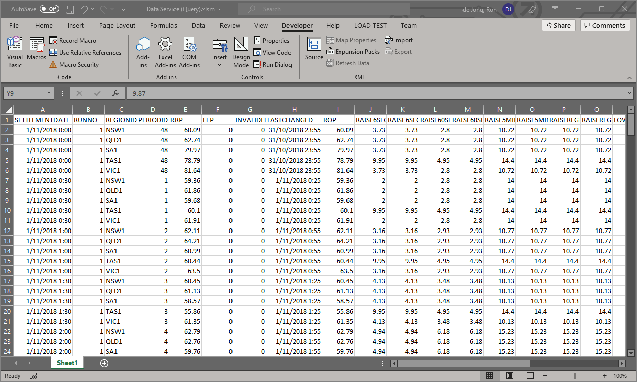
If the above macro is linked to a button and the button is clicked it will load the SQL query results into the spreadsheet as shown below.
MATLAB
MATLAB is a data analysis software package that is very popular amongst engineers and scientists. It has significant enterprise support, so it is often preferred over other open source/free software.
Running reports
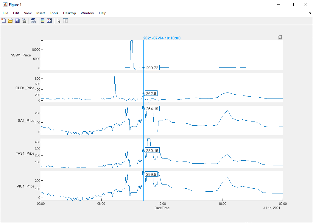
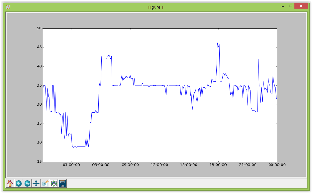
Sample code below loads data from a 5min price report and plots it. Note: the CSV link is obtained from the NEOpoint platform.
url = "https://neopoint.com.au/Service/Csv?f=101+Prices%5CDispatch+and+Predispatch+Prices+5min&from=2021-07-14+00%3A00&period=Daily&instances=§ion=-1&key=******";
data = webread(url);

figure(1)
stackedplot(data, 'XVariable', 'DateTime');
Running SQL queries
To run SQL queries you will need a QueryTool enabled account. Due to the limitation on the length of the GET request url, we have found that is better to use the POST HTTP method to obtain the results from custom queries, especially large queries. The MATLAB code below demonstrates an example where results for a query are downloaded using the POST method.
% Required imports
import matlab.net.http.RequestMessage
import matlab.net.http.field.ContentTypeField
import matlab.net.http.io.FormProvider

% Query to run
query = [
    'select `SETTLEMENTDATE`, `RUNNO`, `REGIONID`, `PERIODID`, `RRP`, `EEP`,'...
    '`INVALIDFLAG`, `LASTCHANGED`, `ROP`, `RAISE6SECRRP`, `RAISE6SECROP`,'...
    '`RAISE60SECRRP`, `RAISE60SECROP`, `RAISE5MINRRP`, `RAISE5MINROP`,'...
    '`RAISEREGRRP`, `RAISEREGROP`, `LOWER6SECRRP`, `LOWER6SECROP`, `LOWER60SECRRP`,'...
    '`LOWER60SECROP`, `LOWER5MINRRP`, `LOWER5MINROP`, `LOWERREGRRP`, `LOWERREGROP`,'...
    '`PRICE_STATUS` from mms.tradingprice where SETTLEMENTDATE between "2018-11-1" and "2018-11-2" limit 0, 10000'
];

% Constructing data payload for message
data = FormProvider('query', query, 'key', '******', 'format', 'csv');

% Constructing POST message
request = RequestMessage( ...
    'POST', ...
    (ContentTypeField( 'application/x-www-form-urlencoded' )), ...
    data ...
);

% Sending Request
response = request.send( 'https://www.neopoint.com.au/data/query' );

% Getting result
result = response.Body.Data;
R Language
R is a very popular open source language based on the S language and used for statistical data analysis. The simplest way to load data is via the CSV format.
Running reports
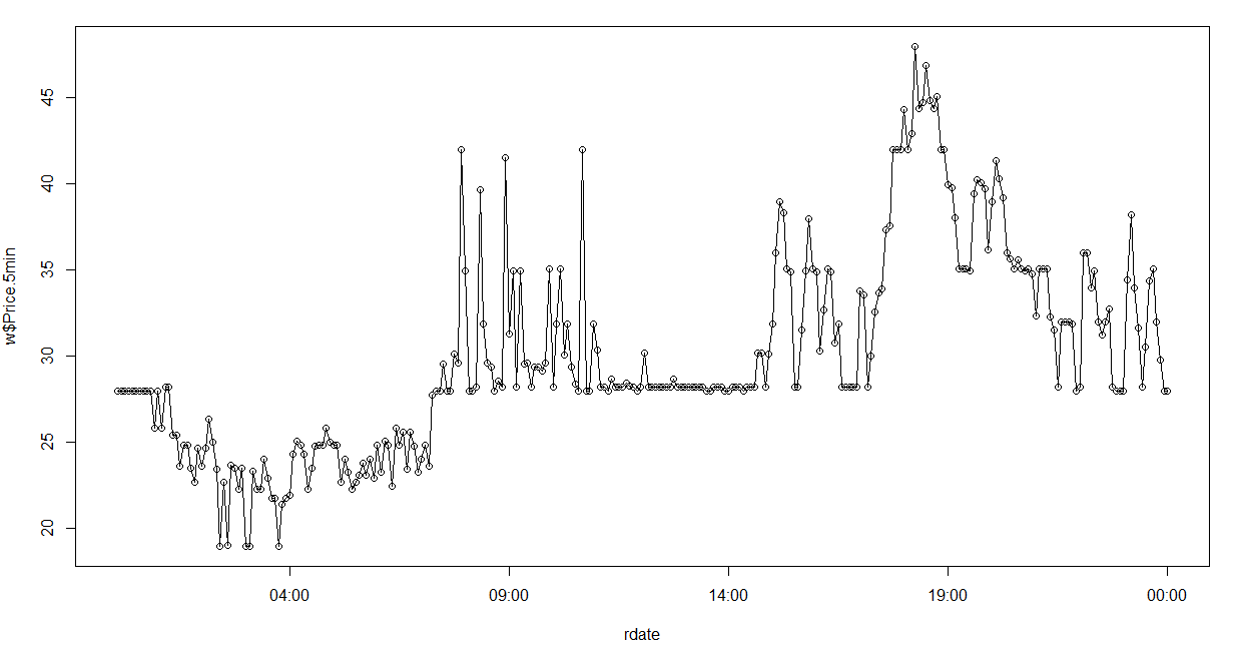
Sample code below loads data from a 5min price report and plots it. Note that this method runs a NEOpoint report rather than an actual query.
w=read.csv(file="https://www.neopoint.com.au/Service/Csv?f=101+Prices%5CDispatch+and+Predispatch+Prices+5min&from=2018-11-05&period=Daily&instances=§ion=-1&key=*****")
plot(w$DateTime, w$NSW1.Price)
lines(w$DateTime, w$NSW1.Price)
rdate<-strptime(w$DateTime, "%Y-%m-%d %H:%M:%S" )
                            plot(rdate, w$NSW1.Price)
                            lines(rdate, w$NSW1.Price)
Running SQL queries
To run SQL queries you need a QueryTool enabled account. Because queries tend to be quite large the HTTP GET method used above cannot be used due to the ~2K limit on the length of a URL, therefore the POST method must be used. The sample code below shows how execute a query. It uses the httr library
library(httr)

query <- "select `SETTLEMENTDATE`, `RUNNO`, `REGIONID`, `PERIODID`, `RRP`, `EEP`,
`INVALIDFLAG`, `LASTCHANGED`, `ROP`, `RAISE6SECRRP`, `RAISE6SECROP`,
`RAISE60SECRRP`, `RAISE60SECROP`, `RAISE5MINRRP`, `RAISE5MINROP`,
`RAISEREGRRP`, `RAISEREGROP`, `LOWER6SECRRP`, `LOWER6SECROP`, `LOWER60SECRRP`,
`LOWER60SECROP`, `LOWER5MINRRP`, `LOWER5MINROP`, `LOWERREGRRP`, `LOWERREGROP`,
`PRICE_STATUS` from mms.tradingprice where SETTLEMENTDATE between '2018-11-1' and '2018-11-2' limit 0, 10000"
         requ <- list(
  query = query,
  key = "*****",
  format="csv"
)
res <- POST("https://www.neopoint.com.au/data/query", body = requ, encode = "form", verbose())
tabtext <- content(res, "text")
tab <- read.csv(text = tabtext, header = TRUE)
The above might look a bit tedious but it is easy to create a function that will wrap all of that up so that running a query just becomes a single function call. In the code sample below we define a function to run a query then we call it. The function takes a query string and returns a data frame.
RunQuery <- function(query) {
            requ <- list(
	  query = query,
	  key = "*****",
	  format="csv"
	)
	res <- POST("https://www.neopoint.com.au/data/query", body = requ, encode = "form", verbose())
	tab <- content(res, "text")
	read.csv(text = tab, header = TRUE)
}

RunQuery("select * from mms.tradingprice where SETTLEMENTDATE between '2018-11-2' and '2018-11-3'")
Python
Python was probably the best of the tools we reviewed! It is a high level scripting language with a very readable syntax making it easier to understand and relay information. It is supported by a very active community of libraries and IDEs and best of all it's free and open source.
Running reports
The Python source code for loading some data from a NEOpoint report and plotting it is shown below. We use the pandas and matplotlib libraries in this example. pandas is a data management and data analysis library and matplotlib is a plotting library; along with numpy, these are some of the most common libraries and come pre-installed in most python distributions.
# Imports import pandas import matplotlib.pyplot as plt # CSV Link url = 'http://neopoint.com.au/service/csv?key=*****§ion=0&f=101+Prices%5cDispatch+Prices+5min&period=Daily&from=2015-04-09&instances=' # Read Data and Plot data = pandas.read_csv(url) data.plot() plt.show()
The chart displayed from the above script is displayed below
Running SQL queries
The Python snippet for loading some data from an SQL query is shown below. Note the code uses the HTTP POST method because the query length will usually exceed the allowed URL length for a GET.
# Imports
import requests
import io
import pandas
import cvs

# Query to run
query = '''select `SETTLEMENTDATE`, `RUNNO`, `REGIONID`, `PERIODID`, `RRP`, `EEP`,
`INVALIDFLAG`, `LASTCHANGED`, `ROP`, `RAISE6SECRRP`, `RAISE6SECROP`,
`RAISE60SECRRP`, `RAISE60SECROP`, `RAISE5MINRRP`, `RAISE5MINROP`,
`RAISEREGRRP`, `RAISEREGROP`, `LOWER6SECRRP`, `LOWER6SECROP`, `LOWER60SECRRP`,
`LOWER60SECROP`, `LOWER5MINRRP`, `LOWER5MINROP`, `LOWERREGRRP`, `LOWERREGROP`,
`PRICE_STATUS` from mms.tradingprice where SETTLEMENTDATE between '2018-11-01' and '2018-11-02' limit 0, 10000'''

# payload for POST request
url = 'https://www.neopoint.com.au/data/query'
data = { 'query': query, 'key':'*****', 'format':'csv'}

# Send HTTP request
response = requests.post(url, data=data)# Note do NOT use params=data as this serialises to the URL!

# Parse the response
data = pandas.read_csv(io.StringIO(response.text),
                  quotechar='\"',
                  delimiter=',',
                  quoting=csv.QUOTE_ALL,
                  skipinitialspace=True,
                  escapechar='\\')

# Remove spaces in the column names
data.columns = data.columns.str.strip()
print (data)
Google Sheets
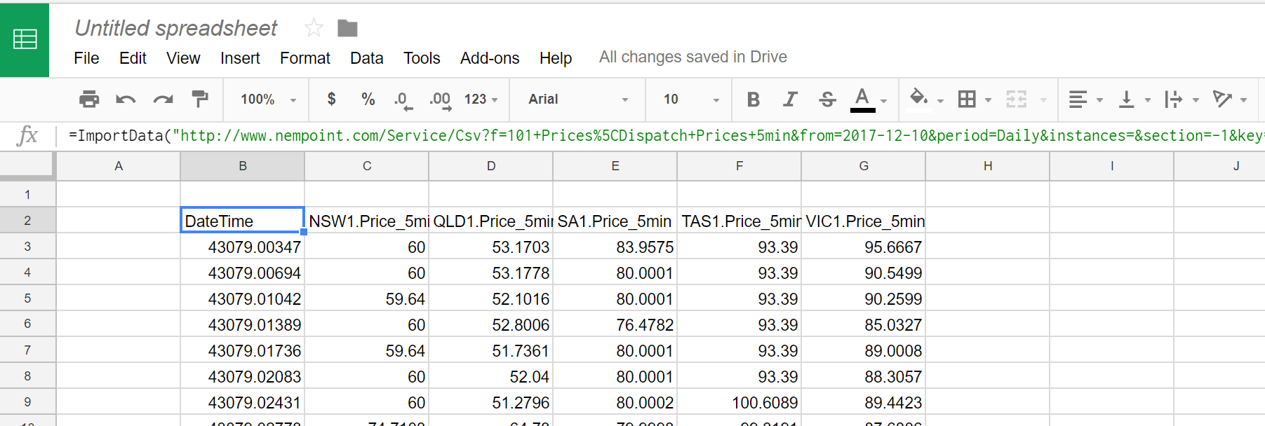
GS can read data in XML or CSV format but we recommend CSV format. The screen shot below shows reading data in by pasting a command like: =ImportData("https://www.neopoint.com.au/Service/Csv?f=101+Prices%5CDispatch+Prices+5min&from=2017-12-10&period=Daily&instances=§ion=-1&key=xxxx")
Alternatively if you want to read the data using a script you can use the sample below as a guide.
function myFunction() {
  var csvUrl = "https://www.neopoint.com.au/Service/Csv?f=101+Prices%5CDispatch+Prices+5min&from=2017-12-10&period=Daily&instances=§ion=-1&key=xxxx";
  var csvContent = UrlFetchApp.fetch(csvUrl).getContentText();
  var csvData = Utilities.parseCsv(csvContent);

  var sheet = SpreadsheetApp.getActiveSheet();
  sheet.getRange(4,4, csvData.length, csvData[0].length).setValues(csvData);
}
Grafana
Grafana is an increasingly popular data visualisation tool used by many organisations to create dashboards for system monitoring and data analysis.
Grafana supports a variety of data formats but the main way to ingest our data is using the JSON links from NEOPoint.
Running Reports
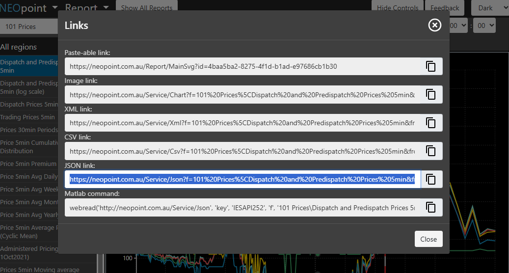
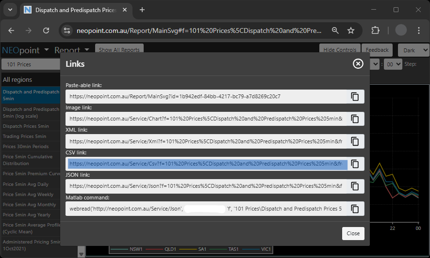
Firstly, find a report in NEOPoint with the desired data and click the links icon:

Then, copy the JSON link to you clipboard and move over to Grafana:
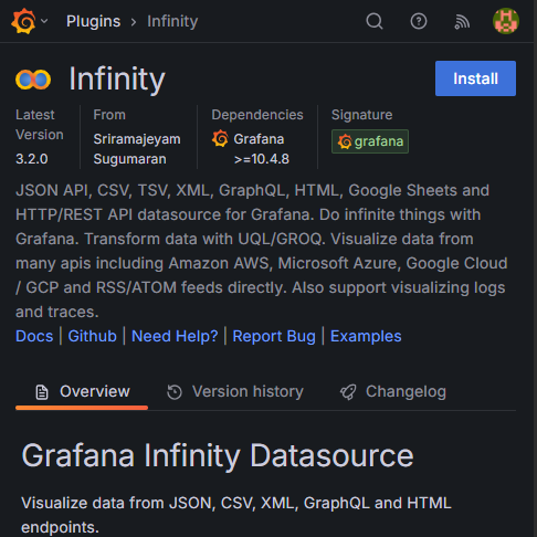
To ingest JSON data make sure you have installed the free Grafana plugin called Infinity Datasource:
Now open up a panel in your dashboard and set the data source to “yesyoreyam-infinity-datasource” and paste the JSON link into the URL field. Also make sure type is set to JSON.
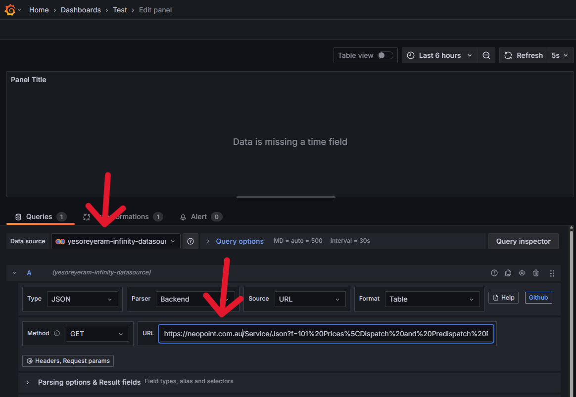
Data should now be viewable under “table view” but wont show as a graph since Grafana doesn’t know the “DateTime” field is a “Time” data type.
To visualise data as a graph you need to add a transformation to the “DateTime” field as shown in the image below:
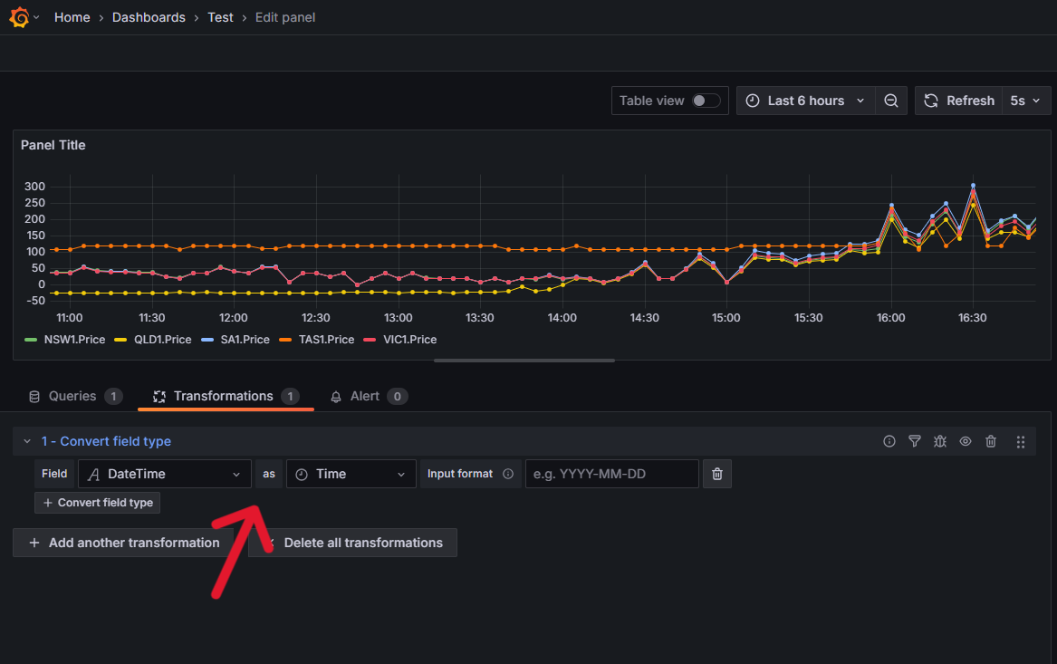
Once the data is visible, you are free to customise the panel using Grafana's extensive configuration options.
Power BI
Our data service also supports integration with Microsoft’s Power BI plataform as it is another popular data visualisation tool.
Running Reports
Importing reports into Power BI is pretty straight forward.
Firstly, in neopoint copy the csv link for your desired report from the links menu.
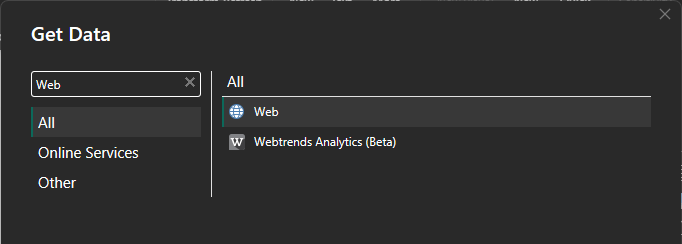
Open Power BI and for the data source select "Web".
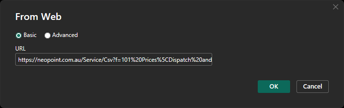
Enter the link you copied from neopoint into the URL field and click OK.
Leave all the default settings and select Load.

Now if the url is valid, under "Table View" on the home page the data should be visible in table format.
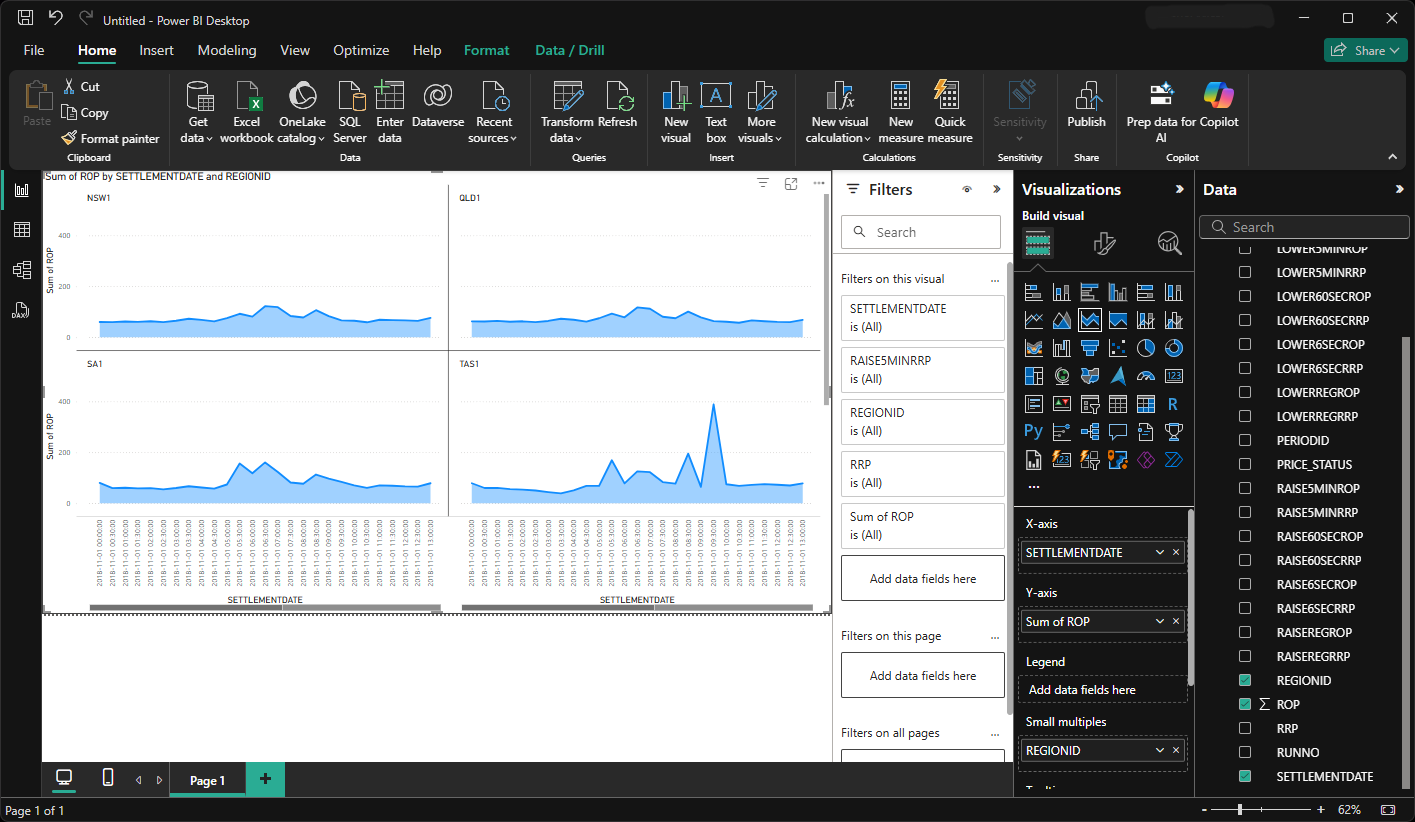
You are now ready to visualise the data in Power BI as you would with any other data.
Running SQL queries
To get data from the data service using an SQL query, first you need to select “Blank Query” for the data source. This will open the Power Query Editor.
![]()
Once the Power Query Editor has loaded, navigate to the "Advanced Editor" which is located under the "View" tab.
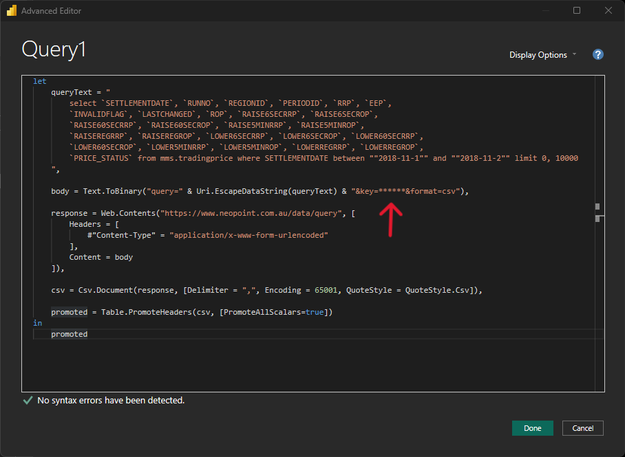
In the "Advanced Editor", enter the desired SQL as follows. (remember to replace the ****** with your API key)
let
    queryText = "
        select `SETTLEMENTDATE`, `RUNNO`, `REGIONID`, `PERIODID`, `RRP`, `EEP`,
        `INVALIDFLAG`, `LASTCHANGED`, `ROP`, `RAISE6SECRRP`, `RAISE6SECROP`,
        `RAISE60SECRRP`, `RAISE60SECROP`, `RAISE5MINRRP`, `RAISE5MINROP`,
        `RAISEREGRRP`, `RAISEREGROP`, `LOWER6SECRRP`, `LOWER6SECROP`, `LOWER60SECRRP`,
        `LOWER60SECROP`, `LOWER5MINRRP`, `LOWER5MINROP`, `LOWERREGRRP`, `LOWERREGROP`,
        `PRICE_STATUS` from mms.tradingprice where SETTLEMENTDATE between ""2018-11-1"" and ""2018-11-2"" limit 0, 10000
    ",
    body = Text.ToBinary("query=" & Uri.EscapeDataString(queryText) & "&key=******&format=csv"),
    response = Web.Contents("https://www.neopoint.com.au/data/query", [
        Headers = [
            #"Content-Type" = "application/x-www-form-urlencoded"
        ],
        Content = body
    ]),
    csv = Csv.Document(response, [Delimiter = ",", Encoding = 65001, QuoteStyle = QuoteStyle.Csv]),
    promoted = Table.PromoteHeaders(csv, [PromoteAllScalars=true])
in
    promoted
If the request is valid, save the query, return to the main screen.
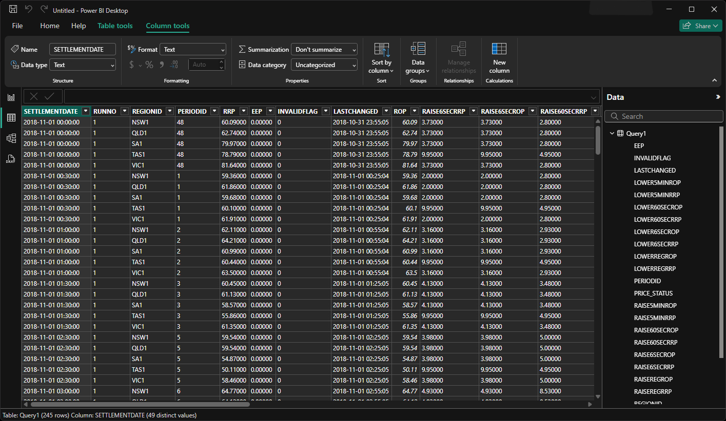
Under "Table View" the data should now be visible in table format.
You are now ready to visualise the data in Power BI as you would with any other data.
IES provides powerful online tools for electricity and gas market data analysis, visualisation and simulation.
+61 2 9436 2555info@iesys.com
www.iesys.com
DATA ANALYSIS
Products / Services
MARKET MODELLING
Product and features
© 2025 Intelligent Energy Systems. All Rights Reserved. | Privacy Policy